Response Curves
Use response curves to inspect the fitted media transformations directly.
Abacus exposes posterior saturation and adstock curves through both the fitted
model and mmm.summary. For decomposition of realised contributions over time,
see Contributions and Decomposition.
Sample saturation curves
Use sample_saturation_curve(...) on a fitted PanelMMM:
The returned xarray.DataArray contains:
- the curve axis
x channel- any panel
dims - a posterior sample dimension
original_scale=True converts the curve’s y-values to original target units.
It does not convert the x-axis. x remains in scaled channel units.
If you want to choose max_value from original channel units, divide by the
relevant value from mmm.data.get_channel_scale().
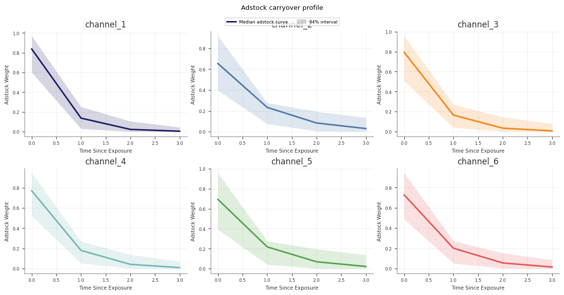
Sample adstock curves
Use sample_adstock_curve(...) to inspect carryover weights:
The returned array contains:
time since exposurechannel- any panel
dims - a posterior sample dimension
The adstock curve is the fitted decay pattern for an impulse of size
amount. It does not use an original_scale option because the returned
weights are not target-unit contributions.
Runner-generated direct contribution artefacts
If you use the retained pipeline runner, Stage 60_response_curves also writes
a forward-pass direct contribution artefact alongside the saturation and
adstock transformation curves:
forward_pass_contribution_curve.ncforward_pass_contribution_curve_summary.csvforward_pass_contribution_curve.png
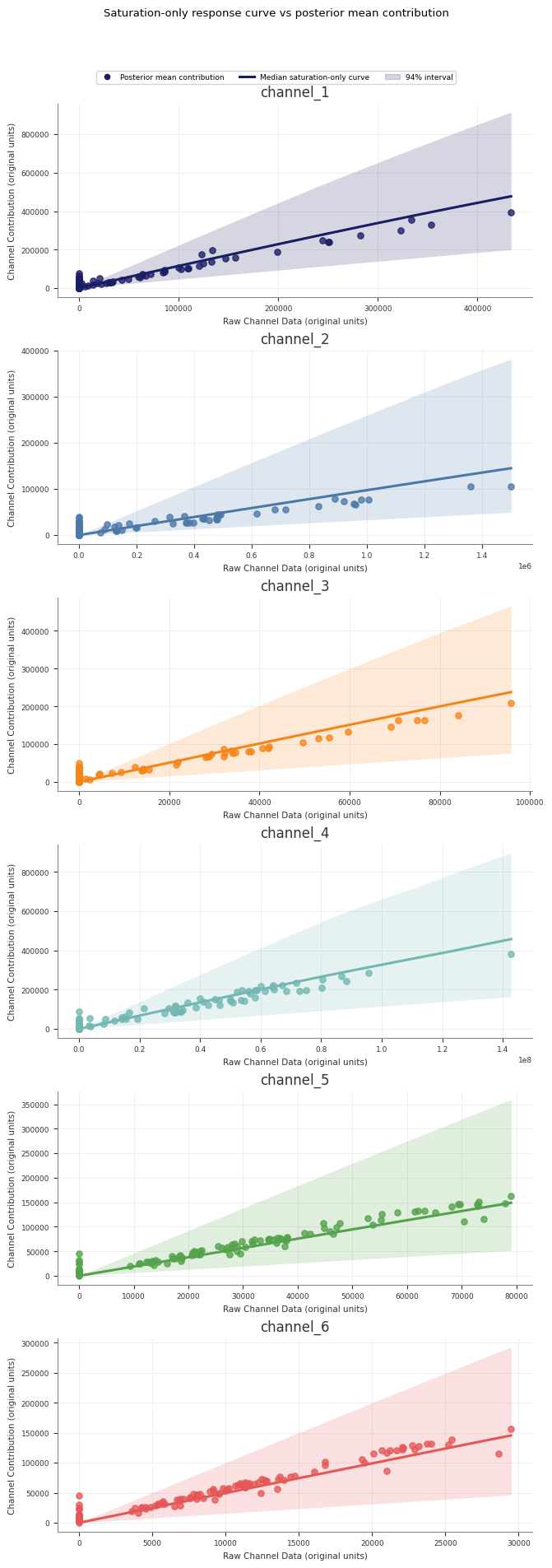
This artefact is different from the saturation-only curve:
- the saturation-only curve shows the fitted saturation transform itself
- the forward-pass direct contribution curve runs spend through the full fitted model path, including adstock and saturation
The retained Stage 60 forward-pass plot uses one explicit scenario so the curve
is interpretable: it rescales the full observed historical spend path from
0% to 200%, then plots total channel spend against total channel
contribution in original units. The marker at 100% highlights the fitted
total contribution for the observed historical spend path.
Summarise curves as DataFrames
If you want tabular summaries, use mmm.summary:
These methods return DataFrames with posterior mean, median, and HDI bound
columns.
saturation_curves(...) includes an x column. adstock_curves(...) uses
time since exposure.
MMMSummaryFactory requirement
Curve summaries need access to both the fitted data and the fitted model transformations.
mmm.summary already satisfies that requirement. If you construct
MMMSummaryFactory manually, pass model=mmm:
If you omit model=mmm, Abacus raises a ValueError.
Plot saturation curves
You can plot sampled curves directly:
You can also inspect the fitted relationship in the observed data with:
Example curve output:
Practical guidance
- Use
num_samplesto trade off speed against posterior resolution. - Use
original_scale=Truewhen you want the saturation y-axis in target units. - Keep in mind that the saturation x-axis stays on the scaled channel axis.
- Use the summary methods when you need exportable tables.
Common pitfalls
- Reading
xfrom saturation curves as original spend units - Forgetting to pass
model=mmmwhen manually constructingMMMSummaryFactory - Comparing adstock curves across models without matching the
amountparameter