It covers posterior predictive checks, diagnostics, contribution analysis,
response curves, efficiency metrics, and the tabular summary surfaces that
Abacus exposes from fitted InferenceData.
Pages
Posterior Predictive: Sample fitted or future
predictions and compare them with observed data where available.
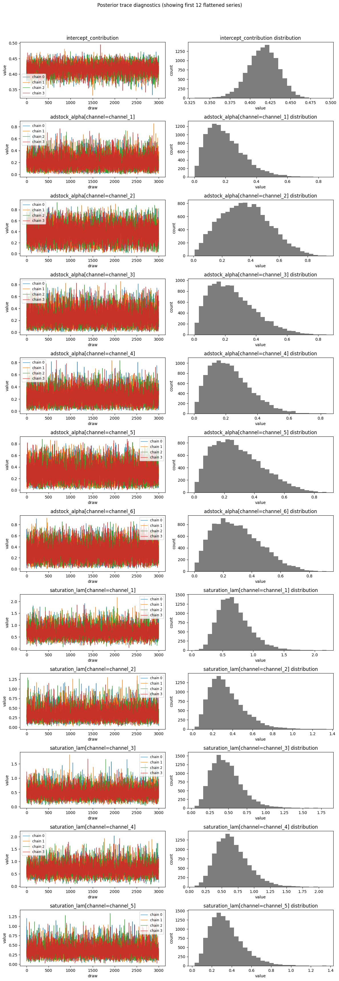
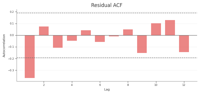
Diagnostics: Run design-matrix, MCMC, and predictive
diagnostics and export machine-readable reports.
Response Curves: Sample and summarise posterior
saturation and adstock curves, and understand the runner’s forward-pass
direct contribution artefacts.
ROAS and Metrics: Calculate ROAS, CPA-style metrics,
spend tables, and predictive error metrics.
Summary and Export: Work with MMMSummaryFactory,
HDI settings, time aggregation, and DataFrame export.
Subsections of Post-Modeling
Diagnostics
Abacus exposes diagnostics through mmm.diagnostics.
Use this surface to check the design matrix, posterior sampling quality, and
posterior predictive fit. For fitted-value plots and predictive sampling, see
Posterior Predictive.
Diagnostic surfaces
mmm.diagnostics provides three groups of checks.
Area
Summary method
Report method
What it covers
Raw input screening
design_summary(X)
design_report(X)
Collinearity, constants, and near-constant regressors on raw input columns
MCMC
mcmc_summary()
mcmc_report()
r_hat, ESS, divergences, BFMI, tree depth, acceptance rate
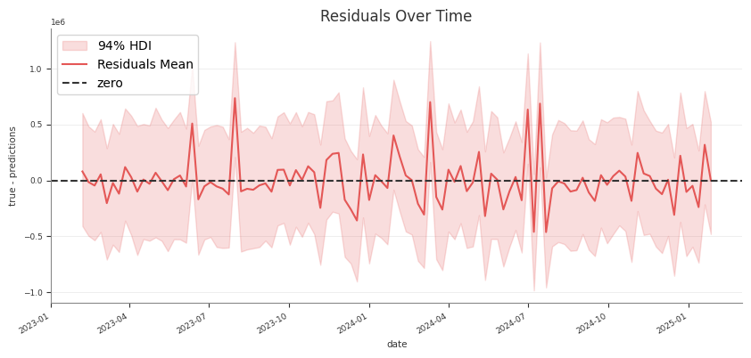
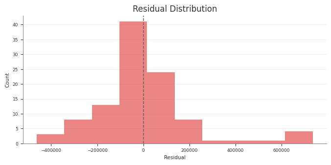
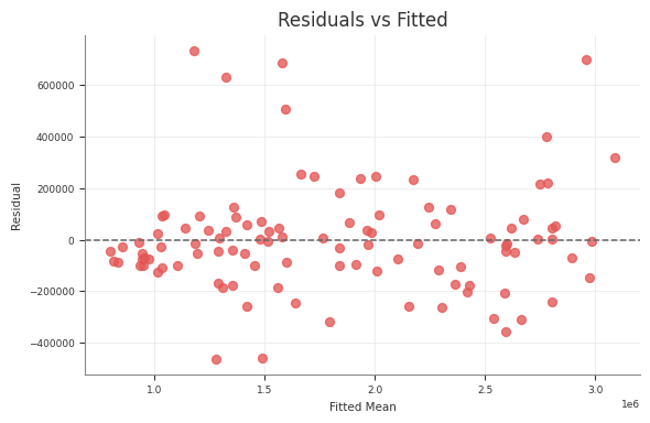
Predictive
predictive_summary()
predictive_report()
RMSE, MAE, NRMSE, NMAE, CRPS, residual moments
The summary methods return pandas DataFrames. The report methods return typed
report objects with a to_dict() method for JSON-ready export.
Raw input screening
Use design_summary(X) on the raw design matrix you want to inspect:
design_report(X) returns a compact roll-up with matrix rank, condition
number, maximum VIF, maximum absolute correlation, and lists of flagged
variables.
Screening requirements
Raw input screening requires:
all requested columns to exist in X
all checked columns to be numeric
Abacus raises a ValueError if a variable is missing or non-numeric.
The method names stay design_summary() and design_report(), but the
pipeline now treats them as raw input screening rather than transformed model
geometry.
The same pattern works for design_report(...) and predictive_report().
Pipeline outputs
The pipeline diagnostics stage uses the same retained diagnostic surfaces to
write report tables and text summaries. If you run the pipeline, those stage
artefacts should match the behaviour documented here.
In the structured pipeline, the raw-input screening rows in
diagnostics_report.csv use the phase label raw_input_screening instead of
design so the machine-readable output matches the wording here.
Common pitfalls
Running mcmc_summary() or mcmc_report() before fitting
Running predictive diagnostics before sampling posterior predictive values
Passing non-numeric columns into design_summary(X)
Treating predictive diagnostics as a substitute for design or MCMC checks
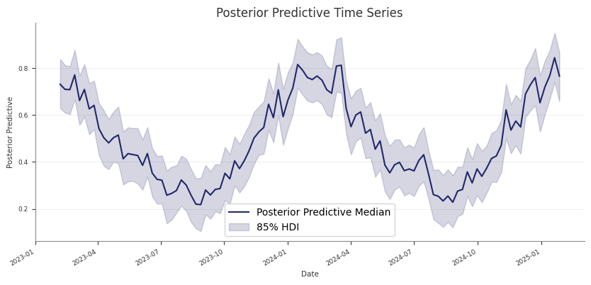
Posterior Predictive Checks
Use posterior predictive draws to check in-sample fit and to generate
predictions for new rows that follow the fitted panel layout.
If you only want the returned samples and do not want to update mmm.idata,
set extend_idata=False.
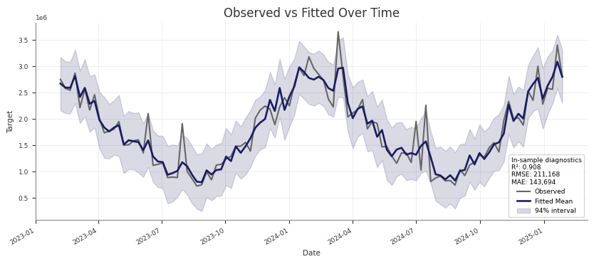
Check training-fit values against observed data
For an in-sample check, pass the same design matrix you used for fitting. This
is the same pattern used by the pipeline’s Stage 30 training-fit assessment:
sample_posterior_predictive(...) does not take y. For a holdout or future
window, keep the actual target outside the model and align it yourself if you
want external evaluation.
Use include_last_observations correctly
Set include_last_observations=True when the forecast window needs lag history
for adstock carryover.
When enabled, Abacus:
prepends the last adstock.l_max training observations internally
samples posterior predictive values on the padded data
removes the prepended rows from the returned result
This only works when the input dates do not overlap with the training dates.
If they do overlap, Abacus raises a ValueError.
Practical guidance
Use the training X for fitted-versus-observed checks.
Use future-only dates for forward prediction.
Use the training-window refit pattern for blocked holdout validation.
Keep combined=True if you want a simpler sample dimension.
Use combined=False if you need explicit chain and draw dimensions.
Call sample_posterior_predictive(...) before using
mmm.diagnostics.predictive_summary() or mmm.summary.posterior_predictive().
Common pitfalls
Calling sample_posterior_predictive(...) without X
Expecting y to be passed into the predictive method
Using include_last_observations=True on dates that overlap with training
data
Forgetting that the returned object is extracted samples, while the stored
idata.posterior_predictive group keeps the native posterior predictive
structure
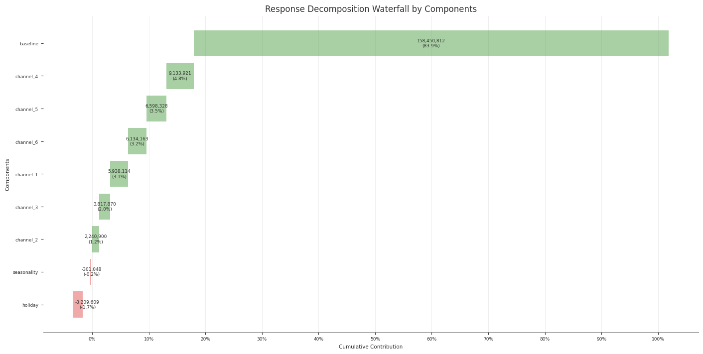
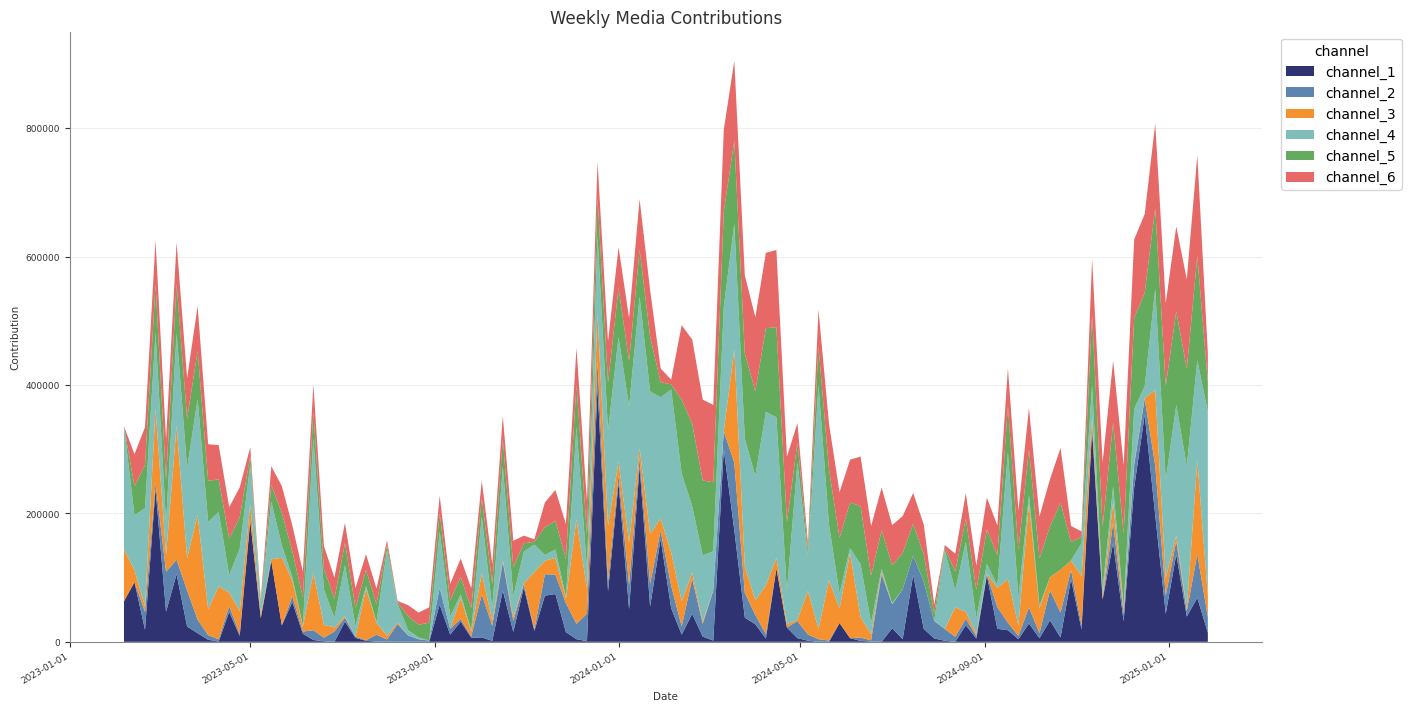
Contributions and Decomposition
Abacus stores additive contribution terms for fitted PanelMMM models and
exposes them through the data wrapper, summary tables, and plotting suite.
Use this page to inspect media, baseline, control, seasonality, and event
effects. For channel efficiency ratios built from media contributions, see
ROAS and Metrics.
Contribution surfaces
You can work with contributions at three levels.
Surface
Use it for
mmm.data
Raw xarray contribution samples
mmm.summary
DataFrames with posterior means, medians, and HDIs
mmm.plot
Time-series and waterfall visualisations
Read raw contribution samples
The lowest-level accessor is mmm.data.get_contributions(...):
identifying columns such as date, channel, control, and any panel
dims
mean
median
HDI bound columns such as abs_error_94_lower and abs_error_94_upper
mmm.summary.contributions(...) does not expose event effects. For event
effects, use mmm.data.get_contributions(include_events=True) or
mmm.summary.mean_contributions_over_time().
Create a wide decomposition table
Use mmm.summary.mean_contributions_over_time(...) when you want one row per
time point and panel slice:
Use original_scale=True when you want business-unit interpretation.
Use mmm.summary.contributions(...) for tidy per-component tables.
Use mmm.summary.mean_contributions_over_time() for decomposition exports.
Use mmm.summary.total_contribution() when you only need component-level
totals.
Common pitfalls
Expecting mmm.summary.contributions(...) to include event effects
Forgetting that baseline can include more than the intercept when Mundlak
CRE is enabled
Using frequency="all_time" with mean_contributions_over_time() or
change_over_time()
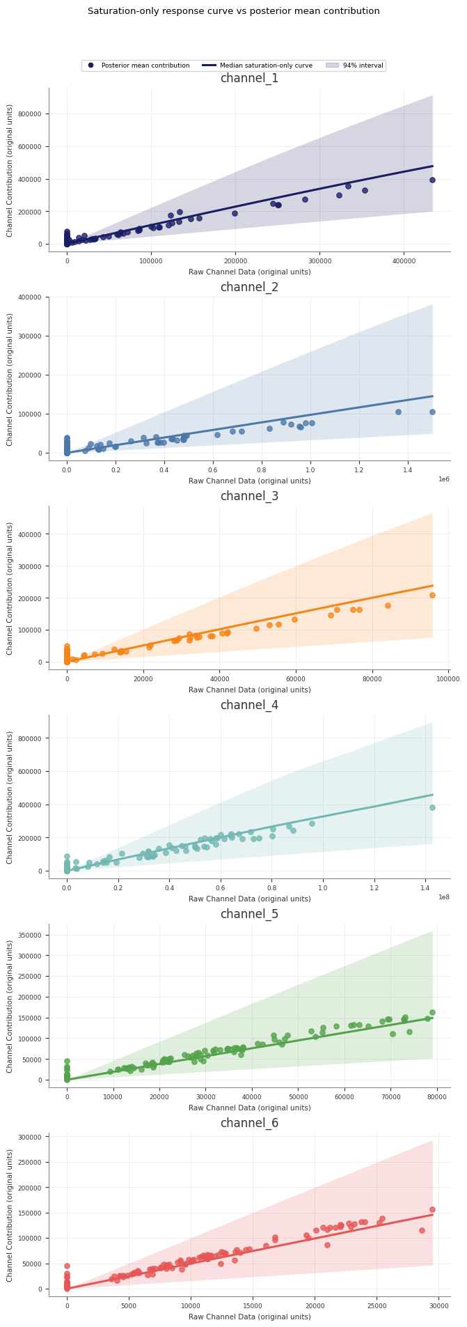
Response Curves
Use response curves to inspect the fitted media transformations directly.
Abacus exposes posterior saturation and adstock curves through both the fitted
model and mmm.summary. For decomposition of realised contributions over time,
see Contributions and Decomposition.
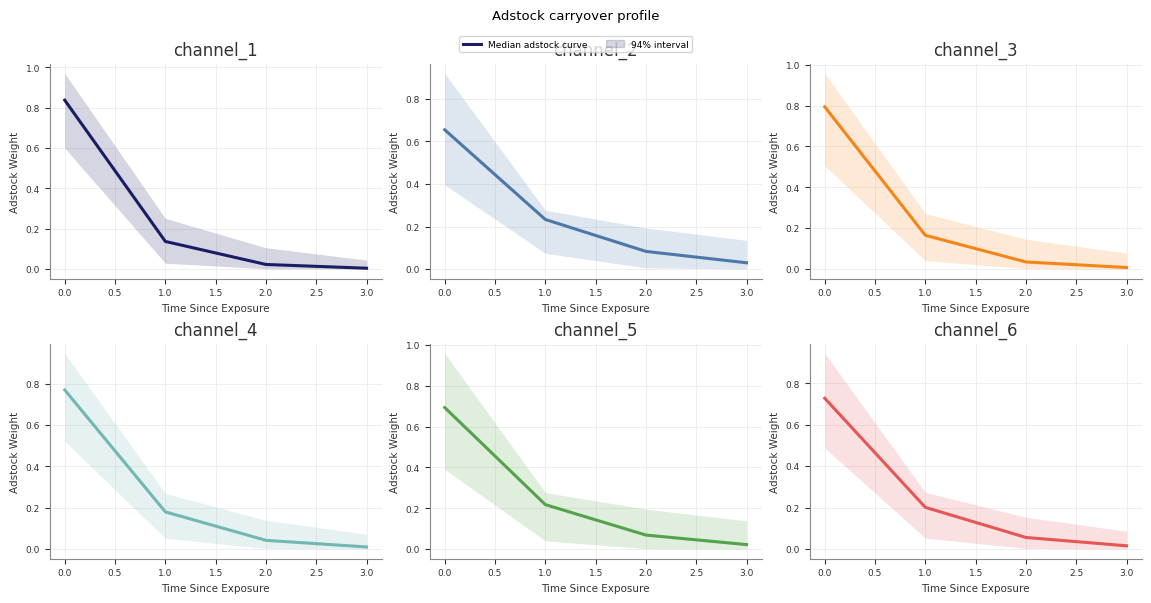
Sample saturation curves
Use sample_saturation_curve(...) on a fitted PanelMMM:
The adstock curve is the fitted decay pattern for an impulse of size
amount. It does not use an original_scale option because the returned
weights are not target-unit contributions.
Runner-generated direct contribution artefacts
If you use the retained pipeline runner, Stage 60_response_curves also writes
a forward-pass direct contribution artefact alongside the saturation and
adstock transformation curves:
forward_pass_contribution_curve.nc
forward_pass_contribution_curve_summary.csv
forward_pass_contribution_curve.png
This artefact is different from the saturation-only curve:
the saturation-only curve shows the fitted saturation transform itself
the forward-pass direct contribution curve runs spend through the full fitted
model path, including adstock and saturation
The retained Stage 60 forward-pass plot uses one explicit scenario so the curve
is interpretable: it rescales the full observed historical spend path from
0% to 200%, then plots total channel spend against total channel
contribution in original units. The marker at 100% highlights the fitted
total contribution for the observed historical spend path.